When the penalized generalize linear model (Lasso or Ridge) is processed in the tidymodel environment, finalizing the hyperparameter (lambda) and getting coefficients of the final model are confusing. Here is an example. This example predicts PIK3CA mutation status by gene expression data. TCGA breast cancer dataset is used.
Modeling
library(glmnet)
library(themis)

set.seed(930093)
cv_splits <- rsample::vfold_cv(trainset_ahDiff, strata = PIK3CA_T)
mod <- logistic_reg(penalty = tune(),
                    mixture = tune()) %>%
  set_engine("glmnet")

rec <- recipe(PIK3CA_T ~ ., data = trainset_ahDiff) %>%
  step_BoxCox(all_numeric()) %>%
  step_dummy(HISTOLOGICAL_DIAGNOSIS) %>%
  step_center(all_numeric()) %>%
  step_scale(all_numeric()) %>%
  step_smote(PIK3CA_T)
wfl <- workflow() %>%
add_recipe(rec) %>%
add_model(mod)
glmn_set <- parameters(penalty(range = c(-5,1), trans = log10_trans()),
mixture())
glmn_grid <-
grid_regular(glmn_set, levels = c(7, 5))
ctrl <- control_grid(save_pred = TRUE, verbose = TRUE)- Grid parameter search on 10-fold cross-validation with 5 repeats
- Dummy variable to control for histologic subtype
Select best parameter
glmn_tune <-
  tune_grid(wfl,
            resamples = cv_splits,
            grid = glmn_grid,
            metrics = metric_set(roc_auc),
            control = ctrl)


best_glmn <- select_best(glmn_tune, metric = "roc_auc")
Finalizing
wfl_final <-
  wfl %>%
  finalize_workflow(best_glmn) %>%
  fit(data = trainset_ahDiff)
finalize_workflow() finalizes the model with selected optimal hyperparameters. However, the glmnet fits any lambda, not the indicated lambda. This was discussed at https://github.com/tidymodels/parsnip/issues/195. The glmnet is more efficient to fit all lambda than a single lambda. Thus tidymodel ignores the indicated lambda. This made the first confusion. The finalization can be finalized by predict in tidymodel environment. Finalize with predict. Note the last argument penalty = 1 of stats::predict(wfl_final, type = "prob", new_data = trainset_ahDiff, penalty = 1).
train_predict <- stats::predict(wfl_final, type = "prob", new_data = trainset_ahDiff, penalty = 1)
train_probs <-
  predict(wfl_final, type = "prob", new_data = trainset_ahDiff) %>%
  bind_cols(obs = trainset_ahDiff$PIK3CA_T) %>%
  bind_cols(predict(wfl_final, new_data = trainset_ahDiff))
Performance
conf_mat(train_probs, obs, .pred_class)## Truth
## Prediction Wild Mutant
## Wild 213 45
## Mutant 123 158autoplot(roc_curve(train_probs, obs, .pred_Mutant, event_level = "second"))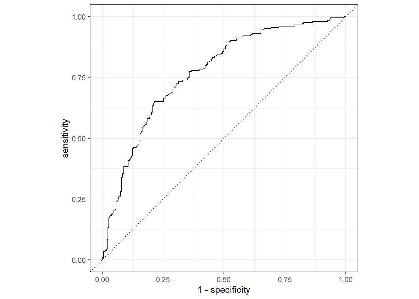
roc_auc(train_probs, obs, .pred_Mutant, event_level = "second")## # A tibble: 1 x 3
## .metric .estimator .estimate
## <chr> <chr> <dbl>
## 1 roc_auc binary 0.770Because glmnet fits the whole path, there are whole coefficients in the glmnet fit object wfl_final. This was the second confusion. How to get the final model coefficients is below.
Coefficients
tidy(extract_model(wfl_final)) %>%
  filter(lambda > 0.98 & lambda < 1.01)
## # A tibble: 17 x 5
## term step estimate lambda dev.ratio
## <chr> <dbl> <dbl> <dbl> <dbl>
## 1 (Intercept) 55 -0.0630 1.00 0.123
## 2 C4A 55 0.0587 1.00 0.123
## 3 C5orf13 55 0.0587 1.00 0.123
## 4 CDSN 55 0.0706 1.00 0.123
## 5 CFB 55 0.0719 1.00 0.123
## 6 CYP21A2 55 0.0516 1.00 0.123
## 7 DGKE 55 -0.0709 1.00 0.123
## 8 FGD5 55 0.0670 1.00 0.123
## 9 GALNT10 55 0.0575 1.00 0.123
## 10 GOLM1 55 0.0689 1.00 0.123
## 11 GPX8 55 0.0657 1.00 0.123
## 12 KLK11 55 0.0145 1.00 0.123
## 13 NTN4 55 0.0578 1.00 0.123
## 14 SMYD3 55 0.0637 1.00 0.123
## 15 USP36 55 -0.0698 1.00 0.123
## 16 WBP2 55 -0.0652 1.00 0.123
## 17 HISTOLOGICAL_DIAGNOSIS_Infiltrating.Lobular.~ 55 -0.0244 1.00 0.123